, ( 2000 2018 ):
() , .
5.9 1 . 2.3 1 . ( 2.6 ).
() , .
( 0.1 - 0.2 ), 2009 . 2011 - 2013 .
, , , 3 ( ).
( 2 18 ). , . 2 ( ).
( ). : , .
" " , ( ).
, .
, , , , , .
, , , , " " (All Offenses) "". , , " " , , , ( ) , . , (, , )... , !
" "
, , ,
df_crimes1 = df_crimes1.loc[df_crimes1['Offense'] == 'All Offenses']:
df_crimes1 = df_crimes1.loc[df_crimes1['Offense'].str.contains('Assault|Murder')], , (Assault) (Murder). , , .
. .
:
, , ( ).
:


:
White_promln_cr | White_promln_uof | Black_promln_cr | Black_promln_uof | |
|---|---|---|---|---|
White_promln_cr | 1.000000 | 0.684757 | 0.986622 | 0.729674 |
White_promln_uof | 0.684757 | 1.000000 | 0.614132 | 0.795486 |
Black_promln_cr | 0.986622 | 0.614132 | 1.000000 | 0.680893 |
Black_promln_uof | 0.729674 | 0.795486 | 0.680893 | 1.000000 |
, (0.68 0.88 0.72 ). , , , .. , .
, "" - :

, . - , .
, .
, - ! :)
, :
, , , : , , . .
51 1991 2018 , :
homicide:
rape legacy: ( - 2013 .)
rape revised: ( - 2013 .)
robbery:
aggravated assault:
property crime:
burglary: /
larceny:
motor vehicle theft:
arson:
(violent crime), .
51 2000 2018 , ( - . ). , 4 (, , ).
:
import pandas as pd, numpy as np

CRIME_STATES_FILE = ROOT_FOLDER + '\\crimes_by_state.csv'
df_crime_states = pd.read_csv(CRIME_STATES_FILE, sep=';', header=0,
                              usecols=['year', 'state_abbr', 'population', 'violent_crime'])
:
year | state_abbr | population | violent_crime | |
|---|---|---|---|---|
0 | 2016 | AL | 4860545 | 25878 |
1 | 1996 | AL | 4273000 | 24159 |
2 | 1997 | AL | 4319000 | 24379 |
3 | 1998 | AL | 4352000 | 22286 |
4 | 1999 | AL | 4369862 | 21421 |
... | ... | ... | ... | ... |
1423 | 2000 | DC | 572059 | 8626 |
1424 | 2001 | DC | 573822 | 9195 |
1425 | 2002 | DC | 569157 | 9322 |
1426 | 2003 | DC | 557620 | 9061 |
1427 | 2016 | DC | 684336 | 8236 |
1428 rows × 4 columns
df_crime_states = df_crime_states.merge(df_state_names, on='state_abbr')
df_crime_states.dropna(inplace=True)
df_crime_states.sort_values(by=['year', 'state_abbr'], inplace=True)
, :
df_crime_states['crime_promln'] = df_crime_states['violent_crime'] * 1e6 / df_crime_states['population'], 2000 2018 , :
df_crime_states_agg = df_crime_states.groupby(['state_name', 'year'])['violent_crime'].sum().unstack(level=1).T
df_crime_states_agg.fillna(0, inplace=True)
df_crime_states_agg = df_crime_states_agg.astype('uint32').loc[2000:2018, :]
19 ( , .. 2000 2018) 51 ( ).
-10 :
df_crime_states_top10 = df_crime_states_agg.describe().T.nlargest(10, 'mean').astype('int32')count | mean | std | min | 25% | 50% | 75% | max | |
|---|---|---|---|---|---|---|---|---|
state_name | ||||||||
California | 19 | 181514 | 19425 | 153763 | 165508 | 178597 | 193022 | 212867 |
Texas | 19 | 117614 | 6522 | 104734 | 113212 | 121091 | 122084 | 126018 |
Florida | 19 | 110104 | 18542 | 81980 | 92809 | 113541 | 127488 | 131878 |
New York | 19 | 81618 | 9548 | 68495 | 75549 | 77563 | 85376 | 105111 |
Illinois | 19 | 62866 | 10445 | 47775 | 54039 | 64185 | 69937 | 81196 |
Michigan | 19 | 49273 | 5029 | 41712 | 44900 | 49737 | 54035 | 56981 |
Pennsylvania | 19 | 46941 | 5066 | 39192 | 41607 | 48188 | 51021 | 55028 |
Tennessee | 19 | 41951 | 2432 | 38063 | 40321 | 41562 | 43358 | 46482 |
Georgia | 19 | 40228 | 3327 | 34355 | 38283 | 39435 | 41495 | 47353 |
North Carolina | 19 | 37936 | 3193 | 32718 | 34706 | 38243 | 40258 | 43125 |
:
df_crime_states_top10 = df_crime_states_agg.loc[:, df_crime_states_agg_top10.index]
plt = df_crime_states_top10.plot.box(figsize=(12, 10))
plt.set_ylabel('-   (2000 - 2018)')
"" . - (, ); :)
, (, , ), (, ).
, . -10 2018 :
df_crime_states_2018 = df_crime_states.loc[df_crime_states['year'] == 2018]
plt = df_crime_states_2018.nlargest(10, 'population').sort_values(by='population').plot.barh(x='state_name', y='population', legend=False, figsize=(10,5))
plt.set_xlabel(' (2018)')
plt.set_ylabel('')
, , . :
#      2000 - 2018  (   )
df_corr = df_crime_states[df_crime_states['year']>=2000].groupby(['state_name']).mean()
#     ""  "- "
df_corr = df_corr.loc[:, ['population', 'violent_crime']]
df_corr.corr(method='pearson').at['population', 'violent_crime']
- 0.98. !
-:
plt = df_crime_states_2018.nlargest(10, 'crime_promln').sort_values(by='crime_promln').plot.barh(x='state_name', y='crime_promln', legend=False, figsize=(10,5))
plt.set_xlabel('-    1 . . (2018)')
plt.set_ylabel('')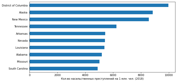
! : (.. ) ( 700+ . 2018 .) (- 2 . .) , , , ...
. folium:
import folium- 2018 . :
FOLIUM_URL = 'https://raw.githubusercontent.com/python-visualization/folium/master/examples/data'
FOLIUM_US_MAP = f'{FOLIUM_URL}/us-states.json'

m = folium.Map(location=[48, -102], zoom_start=3)

folium.Choropleth(
    geo_data=FOLIUM_US_MAP,
    name='choropleth',
    data=df_crime_states_2018,
    columns=['state_abbr', 'violent_crime'],
    key_on='feature.id',
    fill_color='YlOrRd',
    fill_opacity=0.7,
    line_opacity=0.2,
    legend_name='   2018 .',
    bins=df_crime_states_2018['violent_crime'].quantile(list(np.linspace(0.0, 1.0, 5))).to_list(),
    reset=True
).add_to(m)

folium.LayerControl().add_to(m)

m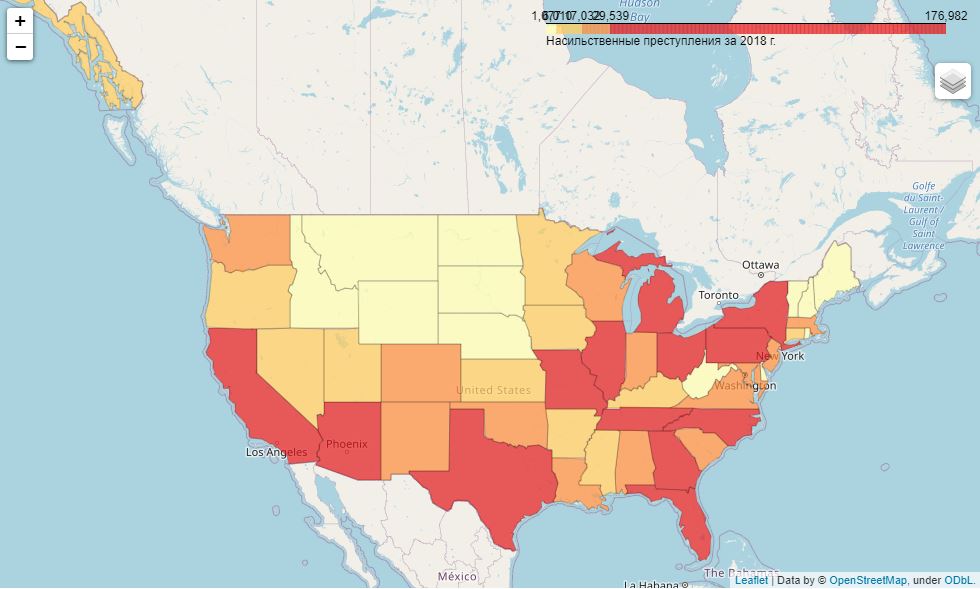
( 1 ):
m = folium.Map(location=[48, -102], zoom_start=3)

folium.Choropleth(
    geo_data=FOLIUM_US_MAP,
    name='choropleth',
    data=df_crime_states_2018,
    columns=['state_abbr', 'crime_promln'],
    key_on='feature.id',
    fill_color='YlOrRd',
    fill_opacity=0.7,
    line_opacity=0.2,
    legend_name='   2018 . ( 1 . )',
    bins=df_crime_states_2018['crime_promln'].quantile(list(np.linspace(0.0, 1.0, 5))).to_list(),
    reset=True
).add_to(m)

folium.LayerControl().add_to(m)

m
, , - .
( )
, .
: (. ) , , 2000 2018 .
df_fenc_agg_states = df_fenc.merge(df_state_names, how='inner', left_on='State', right_on='state_abbr')
df_fenc_agg_states.fillna(0, inplace=True)
df_fenc_agg_states = df_fenc_agg_states.rename(columns={'state_name_x': 'State Name'})
df_fenc_agg_states = df_fenc_agg_states.loc[:, ['Year', 'Race', 'State', 'State Name', 'Cause', 'UOF']]
df_fenc_agg_states = df_fenc_agg_states.groupby(['Year', 'State Name', 'State'])['UOF'].count().unstack(level=0)
df_fenc_agg_states.fillna(0, inplace=True)
df_fenc_agg_states = df_fenc_agg_states.astype('uint16').loc[:, :2018]
df_fenc_agg_states = df_fenc_agg_states.reset_index()
-10 2018 :
df_fenc_agg_states_2018 = df_fenc_agg_states.loc[:, ['State Name', 2018]]
plt = df_fenc_agg_states_2018.nlargest(10, 2018).sort_values(2018).plot.barh(x='State Name', y=2018, legend=False, figsize=(10,5))
plt.set_xlabel('-      2018 .')
plt.set_ylabel('')
" ":
fenc_top10 = df_fenc_agg_states.loc[df_fenc_agg_states['State Name'].isin(df_fenc_agg_states_2018.nlargest(10, 2018)['State Name'])]
fenc_top10 = fenc_top10.T
fenc_top10.columns = fenc_top10.loc['State Name', :]
fenc_top10 = fenc_top10.reset_index().loc[2:, :].set_index('Year')
df_sorted = fenc_top10.mean().sort_values(ascending=False)
fenc_top10 = fenc_top10.loc[:, df_sorted.index]

plt = fenc_top10.plot.box(figsize=(12, 6))
plt.set_ylabel('-     (2000 - 2018)')
, " ": , - . , , , .
, . , .
( ) , 2000 2018 ( ).
#
df_fenc_crime_states = df_fenc.merge(df_state_names, how='inner', left_on='State', right_on='state_abbr')
#
df_fenc_crime_states = df_fenc_crime_states.rename(columns={'Year': 'year', 'state_name_x': 'state_name'})
#    2000-2018
df_fenc_crime_states = df_fenc_crime_states[df_fenc_crime_states['year'].between(2000, 2018)]
#
df_fenc_crime_states = df_fenc_crime_states.groupby(['year', 'state_name'])['UOF'].count().reset_index()
#
df_fenc_crime_states = df_fenc_crime_states.merge(df_crime_states[df_crime_states['year'].between(2000, 2018)], how='outer', on=['year', 'state_name'])
#
df_fenc_crime_states.fillna({'UOF': 0}, inplace=True)
#
df_fenc_crime_states = df_fenc_crime_states.astype({'year': 'uint16', 'UOF': 'uint16', 'population': 'uint32', 'violent_crime': 'uint32'})
#
df_fenc_crime_states = df_fenc_crime_states.sort_values(by=['year', 'state_name'])
:
year | state_name | UOF | state_abbr | population | violent_crime | crime_promln | |
|---|---|---|---|---|---|---|---|
0 | 2000 | Alabama | 7 | AL | 4447100 | 21620 | 4861.595197 |
1 | 2000 | Alaska | 2 | AK | 626932 | 3554 | 5668.876369 |
2 | 2000 | Arizona | 11 | AZ | 5130632 | 27281 | 5317.278651 |
3 | 2000 | Arkansas | 4 | AR | 2673400 | 11904 | 4452.756789 |
4 | 2000 | California | 97 | CA | 33871648 | 210531 | 6215.552311 |
... | ... | ... | ... | ... | ... | ... | ... |
907 | 2018 | Virginia | 18 | VA | 8517685 | 17032 | 1999.604353 |
908 | 2018 | Washington | 24 | WA | 7535591 | 23472 | 3114.818732 |
909 | 2018 | West Virginia | 7 | WV | 1805832 | 5236 | 2899.494527 |
910 | 2018 | Wisconsin | 10 | WI | 5813568 | 17176 | 2954.467893 |
911 | 2018 | Wyoming | 4 | WY | 577737 | 1226 | 2122.072846 |
, UOF ( "Use Of Force" - ) ( "", , ) .
:
df_fenc_crime_states_agg = df_fenc_crime_states.groupby(['state_name']).mean().loc[:, ['UOF', 'violent_crime']]( ):
plt = df_fenc_crime_states_agg['violent_crime'].plot.bar(legend=True, figsize=(15,5))
plt.set_ylabel(' -  ')
plt2 = df_fenc_crime_states_agg['UOF'].plot(secondary_y=True, style='g', legend=True)
plt2.set_ylabel(' -    ', rotation=90)
plt2.set_xlabel('')
plt.set_xlabel('')
plt.set_xticklabels(df_fenc_crime_states_agg.index, rotation='vertical')
plt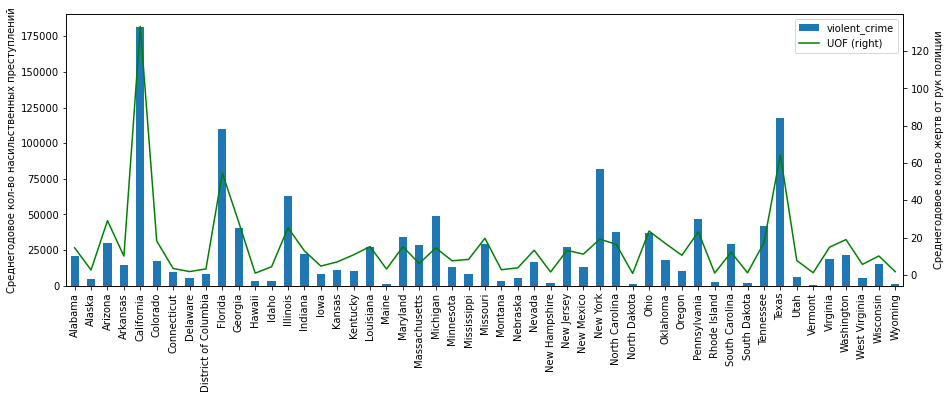
, :
" ": "" ;
(, , , -, ) ( ) .
:
plt = df_fenc_crime_states_agg.plot.scatter(x='violent_crime', y='UOF')
plt.set_xlabel(' -  ')
plt.set_ylabel(' -    ')
, . , 75 . , 75 . "" , , . " ":
df_fenc_crime_states_agg[df_fenc_crime_states_agg['violent_crime'] > 75000]UOF | violent_crime | |
|---|---|---|
state_name | ||
California | 133.263158 | 181514.578947 |
Florida | 54.578947 | 110104.315789 |
New York | 19.157895 | 81618.052632 |
Texas | 64.368421 | 117614.631579 |
, " ": , , -.
3 :
75 .
75 . ( "")
:
df_fenc_crime_states_agg[df_fenc_crime_states_agg['violent_crime'] <= 75000].corr(method='pearson').at['UOF', 'violent_crime']0.839. , 0.9 , 47 .
:
df_fenc_crime_states_agg[df_fenc_crime_states_agg['violent_crime'] > 75000].corr(method='pearson').at['UOF', 'violent_crime']0.999 - !
( ):
df_fenc_crime_states_agg.corr(method='pearson').at['UOF', 'violent_crime']: 0.935. .
, " " (, , ). , , :
df_fenc_crime_states_agg['uof_by_crime'] = df_fenc_crime_states_agg['UOF'] / df_fenc_crime_states_agg['violent_crime']
plt = df_fenc_crime_states_agg.loc[:, 'uof_by_crime'].sort_values(ascending=False).plot.bar(figsize=(15,5))
plt.set_xlabel('')
plt.set_ylabel(' -    - ')
, , , "" ( ).
:
1. (, !)
2. - : , , -.
2. ( ) , , - (. ).
3. , 0.93 . (.. ), - 0.84.
, , , . , , , . , , , , . . , (, , ), .
CSV :
ARRESTS_FILE = ROOT_FOLDER + '\\arrests_by_state_race.csv'
#
df_arrests = pd.read_csv(ARRESTS_FILE, sep=';', header=0, usecols=['data_year', 'state', 'white', 'black'])
#    4
df_arrests = df_arrests.groupby(['data_year', 'state']).sum().reset_index()
#
df_arrests = df_arrests.merge(df_state_names, left_on='state', right_on='state_abbr')
#
df_arrests = df_arrests.rename(columns={'data_year': 'year'}).drop(columns='state_abbr')
# ,
df_arrests.head()
year | state | black | white | state_name | |
|---|---|---|---|---|---|
0 | 2000 | AK | 140 | 613 | Alaska |
1 | 2001 | AK | 139 | 718 | Alaska |
2 | 2002 | AK | 143 | 677 | Alaska |
3 | 2003 | AK | 173 | 801 | Alaska |
4 | 2004 | AK | 163 | 765 | Alaska |
:
df_arrests_agg = df_arrests.groupby(['state_name']).mean().drop(columns='year')51 ( )
black | white | |
|---|---|---|
state_name | ||
Alabama | 2805.842105 | 1757.315789 |
Alaska | 221.894737 | 844.157895 |
Arizona | 1378.368421 | 7007.157895 |
Arkansas | 2387.894737 | 2303.789474 |
California | 26668.368421 | 87252.315789 |
Colorado | 1268.210526 | 5157.368421 |
Connecticut | 2097.631579 | 2981.210526 |
Delaware | 1356.894737 | 1048.578947 |
District of Columbia | 111.111111 | 4.944444 |
Florida | 12.000000 | 7.000000 |
Georgia | 8262.842105 | 3502.894737 |
Hawaii | 81.052632 | 368.736842 |
Idaho | 44.000000 | 1362.263158 |
Illinois | 5699.842105 | 1841.894737 |
Indiana | 3553.368421 | 5192.263158 |
Iowa | 1104.421053 | 3039.473684 |
Kansas | 522.315789 | 1501.315789 |
Kentucky | 1476.894737 | 1906.052632 |
Louisiana | 5928.789474 | 3414.263158 |
Maine | 63.736842 | 699.526316 |
Maryland | 7189.105263 | 4010.684211 |
Massachusetts | 3407.157895 | 7319.684211 |
Michigan | 7628.157895 | 6304.157895 |
Minnesota | 2231.210526 | 2645.736842 |
Mississippi | 1462.210526 | 474.368421 |
Missouri | 5777.473684 | 5703.368421 |
Montana | 27.684211 | 673.684211 |
Nebraska | 591.421053 | 1058.526316 |
Nevada | 1956.421053 | 3817.210526 |
New Hampshire | 68.368421 | 640.789474 |
New Jersey | 6424.157895 | 6043.789474 |
New Mexico | 234.421053 | 2809.368421 |
New York | 8394.526316 | 8734.947368 |
North Carolina | 10527.947368 | 7412.947368 |
North Dakota | 61.263158 | 277.052632 |
Ohio | 4063.947368 | 4071.368421 |
Oklahoma | 1625.105263 | 3353.000000 |
Oregon | 445.105263 | 3373.368421 |
Pennsylvania | 11974.157895 | 11039.473684 |
Rhode Island | 275.684211 | 699.210526 |
South Carolina | 5578.526316 | 3615.421053 |
South Dakota | 67.105263 | 349.368421 |
Tennessee | 6799.894737 | 8462.526316 |
Texas | 10547.631579 | 22062.684211 |
Utah | 167.105263 | 1748.894737 |
Vermont | 43.526316 | 439.210526 |
Virginia | 4100.421053 | 3060.263158 |
Washington | 1688.947368 | 6012.105263 |
West Virginia | 271.263158 | 1528.315789 |
Wisconsin | 3440.055556 | 4107.722222 |
Wyoming | 27.263158 | 506.947368 |
. , - . , , - - 19 (12 7 ). - ; :
df_arrests[df_arrests['state'] == 'FL'], , , 2017 . , , ... . 1-2 . ( ) .
, ( 2000 2009 .) . , 9 ( 2010 2018 .).
POP_STATES_FILES = ROOT_FOLDER + '\\us_pop_states_race_2010-2019.csv'
df_pop_states = pd.read_csv(POP_STATES_FILES, sep=';', header=0)
#    ,   ))
df_pop_states = df_pop_states.melt('state_name', var_name='r_year', value_name='pop')
df_pop_states['race'] = df_pop_states['r_year'].str[0]
df_pop_states['year'] = df_pop_states['r_year'].str[2:].astype('uint16')
df_pop_states.drop(columns='r_year', inplace=True)
df_pop_states = df_pop_states[df_pop_states['year'].between(2000, 2018)]
df_pop_states = df_pop_states.groupby(['state_name', 'year', 'race']).sum().unstack().reset_index()
df_pop_states.columns = ['state_name', 'year', 'black_pop', 'white_pop']
state_name | year | black_pop | white_pop | |
|---|---|---|---|---|
0 | Alabama | 2010 | 5044936 | 13462236 |
1 | Alabama | 2011 | 5067912 | 13477008 |
2 | Alabama | 2012 | 5102512 | 13484256 |
3 | Alabama | 2013 | 5137360 | 13488812 |
4 | Alabama | 2014 | 5162316 | 13493432 |
... | ... | ... | ... | ... |
454 | Wyoming | 2014 | 31392 | 2167008 |
455 | Wyoming | 2015 | 29568 | 2177740 |
456 | Wyoming | 2016 | 29304 | 2170700 |
457 | Wyoming | 2017 | 29444 | 2148128 |
458 | Wyoming | 2018 | 29604 | 2139896 |
1 :
df_arrests_2010_2018 = df_arrests.merge(df_pop_states, how='inner', on=['year', 'state_name'])
df_arrests_2010_2018['white_arrests_promln'] = df_arrests_2010_2018['white'] * 1e6 / df_arrests_2010_2018['white_pop']
df_arrests_2010_2018['black_arrests_promln'] = df_arrests_2010_2018['black'] * 1e6 / df_arrests_2010_2018['black_pop']
:
df_arrests_2010_2018_agg = df_arrests_2010_2018.groupby(['state_name', 'state']).mean().drop(columns='year').reset_index()
df_arrests_2010_2018_agg = df_arrests_2010_2018_agg.set_index('state_name')
( )
state | black | white | black_pop | white_pop | white_arrests_promln | black_arrests_promln | |
|---|---|---|---|---|---|---|---|
state_name | |||||||
Alabama | AL | 1682.000000 | 1342.000000 | 5.152399e+06 | 1.349158e+07 | 99.424741 | 324.055203 |
Alaska | AK | 255.000000 | 870.555556 | 1.069489e+05 | 1.957445e+06 | 445.199704 | 2390.243876 |
Arizona | AZ | 1635.555556 | 6852.000000 | 1.279172e+06 | 2.260403e+07 | 302.923002 | 1267.000192 |
Arkansas | AR | 1960.666667 | 2466.000000 | 1.855574e+06 | 9.465137e+06 | 260.459917 | 1055.854934 |
California | CA | 24381.666667 | 79477.000000 | 1.007921e+07 | 1.128020e+08 | 704.731408 | 2419.234376 |
Colorado | CO | 1377.222222 | 5171.555556 | 9.508173e+05 | 1.882940e+07 | 274.209456 | 1439.257054 |
Connecticut | CT | 1823.777778 | 2295.333333 | 1.643690e+06 | 1.165681e+07 | 196.712775 | 1114.811569 |
Delaware | DE | 1318.000000 | 914.111111 | 8.354622e+05 | 2.635794e+06 | 347.374980 | 1582.395733 |
District of Columbia | DC | 139.222222 | 4.777778 | 1.288488e+06 | 1.154416e+06 | 4.112547 | 108.101938 |
Florida | FL | 12.000000 | 7.000000 | 1.415383e+07 | 6.498292e+07 | 0.107721 | 0.847827 |
Georgia | GA | 8137.222222 | 4271.444444 | 1.279378e+07 | 2.500293e+07 | 170.939250 | 639.869143 |
Hawaii | HI | 81.333333 | 383.777778 | 1.124298e+05 | 1.453712e+06 | 264.353469 | 725.477589 |
Idaho | ID | 51.888889 | 1373.777778 | 5.288222e+04 | 6.154316e+06 | 223.151878 | 978.205026 |
Illinois | IL | 4216.000000 | 1284.222222 | 7.554687e+06 | 3.980927e+07 | 32.199075 | 557.493894 |
Indiana | IN | 2924.444444 | 5186.111111 | 2.522917e+06 | 2.267508e+07 | 228.699515 | 1155.168768 |
Iowa | IA | 1181.000000 | 2999.222222 | 4.305640e+05 | 1.141794e+07 | 262.666753 | 2760.038539 |
Kansas | KS | 539.555556 | 1512.111111 | 7.116182e+05 | 1.006714e+07 | 150.232160 | 758.851182 |
Kentucky | KY | 1443.888889 | 2173.666667 | 1.442174e+06 | 1.558094e+07 | 139.526970 | 1001.433470 |
Louisiana | LA | 5917.000000 | 3255.333333 | 6.021228e+06 | 1.174245e+07 | 277.277874 | 981.334817 |
Maine | ME | 78.000000 | 678.000000 | 7.667733e+04 | 5.059062e+06 | 134.024032 | 1019.061684 |
Maryland | MD | 6460.444444 | 3325.444444 | 7.229037e+06 | 1.426036e+07 | 233.317775 | 893.942720 |
Massachusetts | MA | 3349.555556 | 6895.111111 | 2.249232e+06 | 2.226671e+07 | 309.745910 | 1505.096888 |
Michigan | MI | 6302.444444 | 5647.444444 | 5.645176e+06 | 3.170670e+07 | 178.111684 | 1116.364030 |
Minnesota | MN | 2570.000000 | 2686.777778 | 1.311818e+06 | 1.867259e+07 | 143.902882 | 1986.464052 |
Mississippi | MS | 1251.000000 | 418.777778 | 4.478208e+06 | 7.122651e+06 | 58.753686 | 279.574565 |
Missouri | MO | 4588.333333 | 5146.111111 | 2.854060e+06 | 2.023871e+07 | 254.292323 | 1608.303611 |
Montana | MT | 34.222222 | 788.333333 | 2.210444e+04 | 3.660813e+06 | 214.944902 | 1525.795754 |
Nebraska | NE | 618.888889 | 1154.888889 | 3.701520e+05 | 6.709768e+06 | 172.269972 | 1687.725359 |
Nevada | NV | 2450.000000 | 4480.333333 | 1.052192e+06 | 8.647157e+06 | 517.401564 | 2316.374085 |
New Hampshire | NH | 89.777778 | 784.777778 | 7.873600e+04 | 5.012056e+06 | 156.580888 | 1141.127571 |
New Jersey | NJ | 5429.555556 | 4971.888889 | 5.241910e+06 | 2.595141e+07 | 191.427955 | 1037.217679 |
New Mexico | NM | 260.111111 | 3136.000000 | 2.053876e+05 | 6.905377e+06 | 454.129135 | 1268.115549 |
New York | NY | 6035.777778 | 6600.222222 | 1.373077e+07 | 5.534157e+07 | 119.253616 | 439.581451 |
North Carolina | NC | 9549.000000 | 6759.333333 | 8.804027e+06 | 2.844145e+07 | 238.320077 | 1088.968561 |
North Dakota | ND | 100.666667 | 386.222222 | 6.583289e+04 | 2.583206e+06 | 149.190455 | 1536.987272 |
Ohio | OH | 3632.888889 | 3733.333333 | 5.879375e+06 | 3.844592e+07 | 97.107129 | 617.699379 |
Oklahoma | OK | 1577.333333 | 3049.000000 | 1.189604e+06 | 1.160567e+07 | 262.904593 | 1326.463864 |
Oregon | OR | 375.444444 | 3125.000000 | 3.292284e+05 | 1.402225e+07 | 222.819615 | 1148.158169 |
Pennsylvania | PA | 11227.000000 | 10652.111111 | 5.945100e+06 | 4.232445e+07 | 251.598838 | 1893.415475 |
Rhode Island | RI | 274.888889 | 595.000000 | 3.275551e+05 | 3.592825e+06 | 165.605635 | 837.932682 |
South Carolina | SC | 4703.222222 | 3094.111111 | 5.365012e+06 | 1.324712e+07 | 234.287821 | 877.892998 |
South Dakota | SD | 103.777778 | 448.333333 | 6.154533e+04 | 2.903489e+06 | 153.995184 | 1641.137012 |
Tennessee | TN | 7603.000000 | 9068.666667 | 4.460808e+06 | 2.070126e+07 | 438.486812 | 1708.022356 |
Texas | TX | 10821.666667 | 21122.111111 | 1.345661e+07 | 8.628389e+07 | 245.051258 | 803.917061 |
Utah | UT | 193.222222 | 1797.333333 | 1.558876e+05 | 1.079659e+07 | 166.431266 | 1240.117890 |
Vermont | VT | 54.222222 | 520.555556 | 3.017111e+04 | 2.376143e+06 | 219.129918 | 1785.111547 |
Virginia | VA | 4059.555556 | 3071.222222 | 6.544598e+06 | 2.340732e+07 | 131.178648 | 620.504151 |
Washington | WA | 1791.777778 | 5870.444444 | 1.147000e+06 | 2.289368e+07 | 256.632241 | 1566.862244 |
West Virginia | WV | 294.111111 | 1648.666667 | 2.597649e+05 | 6.908718e+06 | 238.517207 | 1132.059057 |
Wisconsin | WI | 3525.333333 | 4046.222222 | 1.516534e+06 | 2.018658e+07 | 200.441064 | 2325.622492 |
Wyoming | WY | 28.777778 | 464.555556 | 2.856356e+04 | 2.151349e+06 | 216.004646 | 1005.725503 |
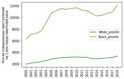
:
plt = df_arrests_2010_2018_agg.loc[:, ['white', 'black']].sort_index(ascending=False).plot.barh(color=['g', 'olive'], figsize=(10, 20))
plt.set_ylabel('')
plt.set_xlabel(' -  (2010-2018 .)')

2. :
plt = df_arrests_2010_2018_agg.loc[:, ['white_arrests_promln', 'black_arrests_promln']].sort_index(ascending=False).plot.barh(color=['g', 'olive'], figsize=(10, 20))
plt.set_ylabel('')
plt.set_xlabel(' -   1    (2010-2018 .)')
?
-, , - .
-, . "", , (. , , , .) -, ( , , , , , .
-, ( ) , .
.
:
df_arrests_2010_2018['white'].mean() / df_arrests_2010_2018['black'].mean()- 1.56. .. 9 , .
:
df_arrests_2010_2018['white_arrests_promln'].mean() / df_arrests_2010_2018['black_arrests_promln'].mean()- 0.183. .. 5.5 , .
, .
, , .
:
df_fenc_agg_states1 = df_fenc.merge(df_state_names, how='inner', left_on='State', right_on='state_abbr')
df_fenc_agg_states1.fillna(0, inplace=True)
df_fenc_agg_states1 = df_fenc_agg_states1.rename(columns={'state_name_x': 'state_name', 'Year': 'year'})
df_fenc_agg_states1 = df_fenc_agg_states1.loc[df_fenc_agg_states1['year'].between(2000, 2018), ['year', 'Race', 'state_name', 'UOF']]
df_fenc_agg_states1 = df_fenc_agg_states1.groupby(['year', 'state_name', 'Race'])['UOF'].count().unstack().reset_index()
df_fenc_agg_states1 = df_fenc_agg_states1.rename(columns={'Black': 'black_uof', 'White': 'white_uof'})
df_fenc_agg_states1 = df_fenc_agg_states1.fillna(0).astype({'black_uof': 'uint32', 'white_uof': 'uint32'})
year | state_name | black_uof | white_uof | |
|---|---|---|---|---|
0 | 2000 | Alabama | 4 | 3 |
1 | 2000 | Alaska | 0 | 2 |
2 | 2000 | Arizona | 0 | 11 |
3 | 2000 | Arkansas | 1 | 3 |
4 | 2000 | California | 19 | 78 |
... | ... | ... | ... | ... |
907 | 2018 | Virginia | 11 | 7 |
908 | 2018 | Washington | 0 | 24 |
909 | 2018 | West Virginia | 2 | 5 |
910 | 2018 | Wisconsin | 3 | 7 |
911 | 2018 | Wyoming | 0 | 4 |
:
df_arrests_fenc = df_arrests.merge(df_fenc_agg_states1, on=['state_name', 'year'])
df_arrests_fenc = df_arrests_fenc.rename(columns={'white': 'white_arrests', 'black': 'black_arrests'})
2017
year | state | black_arrests | white_arrests | state_name | black_uof | white_uof | |
|---|---|---|---|---|---|---|---|
15 | 2017 | AK | 266 | 859 | Alaska | 2 | 3 |
34 | 2017 | AL | 3098 | 2509 | Alabama | 7 | 17 |
53 | 2017 | AR | 2092 | 2674 | Arkansas | 6 | 7 |
72 | 2017 | AZ | 2431 | 7829 | Arizona | 6 | 43 |
91 | 2017 | CA | 24937 | 80367 | California | 25 | 137 |
110 | 2017 | CO | 1781 | 6079 | Colorado | 2 | 27 |
127 | 2017 | CT | 1687 | 2114 | Connecticut | 1 | 5 |
140 | 2017 | DE | 1198 | 782 | Delaware | 4 | 3 |
159 | 2017 | GA | 7747 | 4171 | Georgia | 15 | 21 |
173 | 2017 | HI | 88 | 419 | Hawaii | 0 | 1 |
192 | 2017 | IA | 1400 | 3524 | Iowa | 1 | 5 |
210 | 2017 | ID | 61 | 1423 | Idaho | 0 | 6 |
229 | 2017 | IL | 2847 | 947 | Illinois | 13 | 11 |
248 | 2017 | IN | 3565 | 4300 | Indiana | 9 | 13 |
267 | 2017 | KS | 585 | 1651 | Kansas | 3 | 10 |
286 | 2017 | KY | 1481 | 2035 | Kentucky | 1 | 18 |
305 | 2017 | LA | 5875 | 2284 | Louisiana | 13 | 5 |
324 | 2017 | MA | 2953 | 6089 | Massachusetts | 1 | 4 |
343 | 2017 | MD | 6662 | 3371 | Maryland | 8 | 5 |
361 | 2017 | ME | 89 | 675 | Maine | 1 | 8 |
380 | 2017 | MI | 6149 | 5459 | Michigan | 6 | 7 |
399 | 2017 | MN | 2513 | 2681 | Minnesota | 1 | 7 |
418 | 2017 | MO | 4571 | 5007 | Missouri | 13 | 20 |
437 | 2017 | MS | 1266 | 409 | Mississippi | 7 | 10 |
455 | 2017 | MT | 50 | 915 | Montana | 0 | 3 |
474 | 2017 | NC | 8177 | 5576 | North Carolina | 9 | 14 |
501 | 2017 | NE | 80 | 578 | Nebraska | 0 | 1 |
516 | 2017 | NH | 113 | 817 | New Hampshire | 0 | 3 |
535 | 2017 | NJ | 4859 | 4136 | New Jersey | 9 | 6 |
554 | 2017 | NM | 205 | 2094 | New Mexico | 0 | 20 |
573 | 2017 | NV | 2695 | 4657 | Nevada | 3 | 12 |
592 | 2017 | NY | 5923 | 6633 | New York | 7 | 9 |
611 | 2017 | OH | 4472 | 3882 | Ohio | 11 | 23 |
630 | 2017 | OK | 1638 | 2872 | Oklahoma | 3 | 20 |
649 | 2017 | OR | 453 | 3222 | Oregon | 2 | 9 |
668 | 2017 | PA | 10123 | 10191 | Pennsylvania | 7 | 17 |
681 | 2017 | RI | 315 | 633 | Rhode Island | 0 | 1 |
700 | 2017 | SC | 4645 | 2964 | South Carolina | 3 | 10 |
712 | 2017 | SD | 124 | 537 | South Dakota | 0 | 2 |
731 | 2017 | TN | 6654 | 8496 | Tennessee | 4 | 24 |
750 | 2017 | TX | 11493 | 20911 | Texas | 18 | 56 |
769 | 2017 | UT | 199 | 1964 | Utah | 1 | 5 |
788 | 2017 | VA | 4283 | 3247 | Virginia | 8 | 17 |
804 | 2017 | VT | 75 | 626 | Vermont | 0 | 1 |
823 | 2017 | WA | 1890 | 5804 | Washington | 8 | 27 |
842 | 2017 | WV | 350 | 1705 | West Virginia | 1 | 10 |
856 | 2017 | WY | 36 | 549 | Wyoming | 0 | 1 |
872 | 2017 | DC | 135 | 8 | District of Columbia | 1 | 1 |
890 | 2017 | WI | 3604 | 4106 | Wisconsin | 6 | 15 |
892 | 2017 | FL | 12 | 7 | Florida | 19 | 43 |
, , :
df_corr = df_arrests_fenc.loc[:, ['white_arrests', 'black_arrests', 'white_uof', 'black_uof']].corr(method='pearson').iloc[:2, 2:]
df_corr.style.background_gradient(cmap='PuBu')
white_uof | black_uof | |
|---|---|---|
white_arrests | 0.872766 | 0.622167 |
black_arrests | 0.702350 | 0.766852 |
: 0.87 0.77 ! , , ( 0.88 0.72 ).
, " ", :
df_arrests_fenc['white_uof_by_arr'] = df_arrests_fenc['white_uof'] / df_arrests_fenc['white_arrests']
df_arrests_fenc['black_uof_by_arr'] = df_arrests_fenc['black_uof'] / df_arrests_fenc['black_arrests']
df_arrests_fenc.replace([np.inf, -np.inf], np.nan, inplace=True)
df_arrests_fenc.fillna({'white_uof_by_arr': 0, 'black_uof_by_arr': 0}, inplace=True)
, ( 2018 ):
plt = df_arrests_fenc.loc[df_arrests_fenc['year'] == 2018, ['state_name', 'white_uof_by_arr', 'black_uof_by_arr']].sort_values(by='state_name', ascending=False).plot.barh(x='state_name', color=['g', 'olive'], figsize=(10, 20))
plt.set_ylabel('')
plt.set_xlabel(' -   -  ( 2018 .)')
, , : , , , .
:
plt = df_arrests_fenc.loc[:, ['white_uof_by_arr', 'black_uof_by_arr']].mean().plot.bar(color=['g', 'olive'])
plt.set_ylabel(' -   - ')
plt.set_xticklabels(['', ''], rotation=0)
2.5 . , - , 2.5 , . , : , 2 , - 4 .
, . .
. "" , , - . ( ) - , ( ) -.
( ), .
: 3 5 , .
2.5 , .
: , . , . : , .
, :)
PS. , . , . , !