Hello Habr! Como profissão principal, sou engenheiro de desenvolvimento de campos de petróleo e gás. Estou mergulhando no Data Sciense e esta é minha primeira postagem em que gostaria de compartilhar minha experiência com aprendizado de máquina na indústria de petróleo.

. , , .
. , ( ).
, . .
:
( + ) () () , .
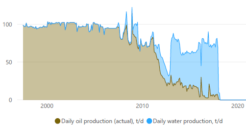
( ). () . , , - - , .
, , . .
3D ().
, ( ). . , . . . . 10 - 15 . , 3- 250 - 1000 . , , " ".
. . . - , . - 3- ( , ) ( ). . , .
. .
:
( , , /- , , ..),
- , , .
. . , . , . , - . .. Q/(Q + Q)*100%
( ) :
:
Cum oil:
Days: ( ( ) ).
In prod: /
Q oil:
wct:
Top perf: -
Bottom perf:
ST: 0 - , 1 -
x, y:
import numpy as np
import pandas as pd
import matplotlib.pyplot as plt
%matplotlib inline
%config InlineBackend.figure_format = 'svg'
import pylab
from pylab import rcParams
import plotly.express as px
import plotly.graph_objects as go
from sklearn.model_selection import train_test_split
from sklearn.ensemble import RandomForestRegressor
from sklearn.metrics import r2_score as r2, mean_absolute_error as mae, mean_squared_error as mse, accuracy_score
from sklearn.metrics.pairwise import euclidean_distances
.
data_path = 'art_df.xlsx'
df = pd.read_excel(data_path, sheet_name='artificial')
df

- . ( ).
ax = df.plot(kind='scatter', x='x', y='y')
df[['x','y','Well']].apply(lambda row: ax.text(*row),axis=1);
rcParams['figure.figsize'] = [11, 8]
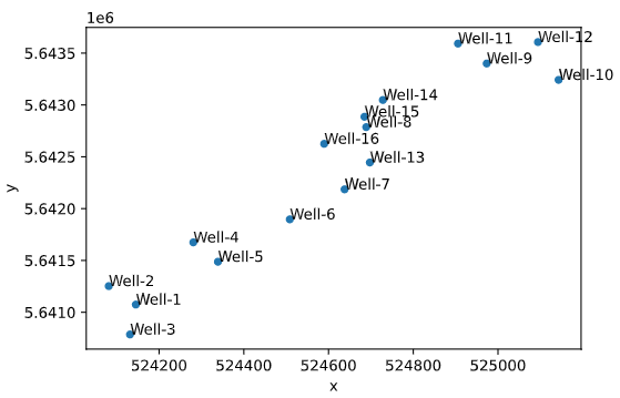
, " " . . , , .
.
distance = pd.DataFrame(euclidean_distances(df[['x', 'y']]))
distance
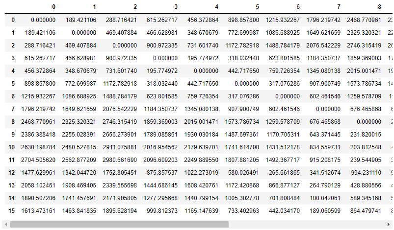
. .
well_names = df['Well']
distance.columns = well_names
. - , .
df_distance = pd.concat([df.drop(['x', 'y'], axis=1), distance], axis=1)
df_distance
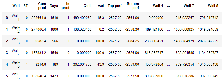
. , ,
df_train_1 = df_distance.drop([12, 13, 14, 15], axis=0)
df_train_1

df_test_1 = df_distance.loc[[12, 13]]
df_test_1

DataFrame X_1. ( ) wct.
x_1 = df_train_1.drop(['Well', 'wct'], axis=1)
x_1

y_1
y_1 = df_train_1['wct']
y_test_1
y_test_1 = df_test_1['wct']
Random Forest Reggressor, , .
x_test_1 = df_test_1.drop(['Well', 'wct'], axis=1)
model = RandomForestRegressor(random_state=42, max_depth=14)
model.fit(x_1, y_1)
y_pred_train_1 = model.predict(x_1)
y_pred_1 = model.predict(x_test_1)
print('Predicted values from train data:')
r2_train = r2(y_1, y_pred_train_1)
mae_train = mae(y_1, y_pred_train_1)
mse_train = mse(y_1, y_pred_train_1)
print(f'R2 train: {r2_train.round(4)}')
print(f'MAE train: {mae_train.round(4)}')
print(f'MSE train: {mse_train.round(4)}')
print('Predicted values from test data:')
r2_test = r2(y_test_1, y_pred_1)
mae_test = mae(y_test_1, y_pred_1)
mse_test = mse(y_test_1, y_pred_1)
print(f'R2 test: {r2_test.round(4)}')
print(f'MAE test: {mae_test.round(4)}')
print(f'MSE test: {mse_test.round(4)}')
model
Predicted values from train data:
R2 train: 0.8832
MAE train: 8.2855
MSE train: 131.1208
Predicted values from test data:
R2 test: 0.8758
MAE test: 3.164
MSE test: 11.4485
RandomForestRegressor(max_depth=14, random_state=42)
R2 R2 1%. , .
, (blind test)
df_y_test = pd.DataFrame({'Well': df_test_1['Well'],
'wct predicted, %': y_pred_1.round(1),
'wct actual, %': y_test_1.round(1),
'difference': (y_pred_1 - y_test_1).round(1)})
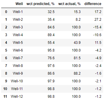
df_y_test

df_y_train = pd.DataFrame({'Well': df_train_1['Well'],
'wct predicted, %': y_pred_train_1.round(1),
'wct actual, %': y_1.round(1),
'difference': (y_pred_train_1 - y_1).round(1)})
df_y_train
:
round(sum(abs(y_pred_train_1 - y_1)) / len(y_1), 1)
8.3
, 8%, .
, ,
df_train_2 = df_distance.drop([14, 15], axis=0)
, .
WCT () = NaN.
df_fc = df_distance.loc[[14, 15]]
DataFrame x_2. ( ) wct.
x_2 = df_train_2.drop(['Well', 'wct'], axis=1)
y_2 .
y_2 = df_train_2['wct']
x_fc = df_fc.drop(['Well', 'wct'], axis=1)
model = RandomForestRegressor(random_state=42, max_depth=14)
model.fit(x_2, y_2)
y_pred_train_2 = model.predict(x_2)
y_fc = model.predict(x_fc)
print('Predicted values from train data:')
r2_train = r2(y_2, y_pred_train_2)
mae_train = mae(y_2, y_pred_train_2)
mse_train = mse(y_2, y_pred_train_2)
print(f'R2 train: {r2_train.round(4)}')
print(f'MAE train: {mae_train.round(4)}')
print(f'MSE train: {mse_train.round(4)}')
print('Forecasted values could be compared with real data!')
model
Predicted values from train data:
R2 train: 0.9095
MAE train: 6.5196
MSE train: 89.9625
RandomForestRegressor(max_depth=14, random_state=42)
R2 .
.
df_y_train = pd.DataFrame({'Well': df_train_2['Well'],
'wct predicted, %': y_pred_train_2.round(1),
'wct actual, %': y_2.round(1),
'difference': (y_pred_train_2 - y_2).round(1)})
df_y_train
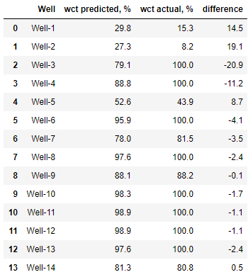
round(sum(abs(y_pred_train_2 - y_2)) / len(y_2), 1)
6,5
6,5. !
:
df_y_test = pd.DataFrame({'Well': df_test_1['Well'],
'wct predicted, %': y_pred_1.round(1),
'wct actual, %': y_test_1.round(1),
'difference': (y_pred_1 - y_test_1).round(1)})
df_y_test

.
model.feature_importances_
feature_importances = pd.DataFrame()
feature_importances['feature_name'] = x_2.columns.tolist()
feature_importances['importance'] = model.feature_importances_
feature_importances = feature_importances.sort_values(by='importance', ascending=False)
feature_importances
fig = px.bar(feature_importances,
x=feature_importances['importance'],
y=feature_importances['feature_name'],
title="Feature importances")
fig.update_layout(yaxis={'categoryorder':'total ascending'})
fig.show()
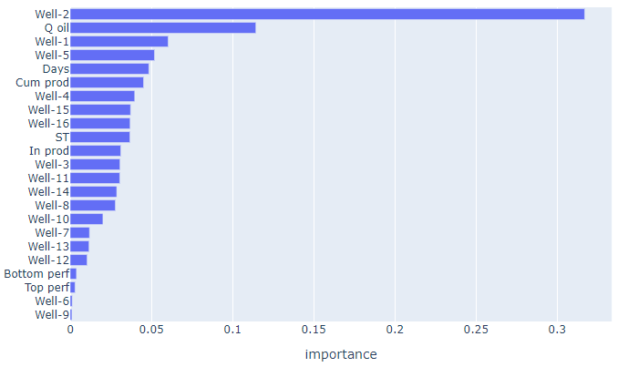
, - 2- . .
. - .
fig = px.scatter(x=y_pred_train_2, y=y_2, title="True vs Predicted values",
text=df_train_2['Well'], width=850, height=800)
fig.add_trace(go.Scatter(x=[0,100], y=[0,100], mode='lines', name='True=Predicted',
line = dict(color='red', width=1, dash='dash')))
fig.update_xaxes(title_text='Predicted')
fig.update_yaxes(title_text='True')
fig.show()

. (- ), (, ).
, " " . , , .
. - "" - .

. " ", . "" . . , .
, . , .
Os dados do poço não são dados abertos, mas sim propriedade da empresa que detém a licença para desenvolver o campo. Portanto, para ilustrar o trabalho realizado, foram gerados dados de poços artificiais que estão disponíveis para este trabalho.
O código-fonte junto com o texto do artigo está disponível aqui: https://github.com/alex-kalinichenko/re/tree/master/wct_fc