A tradução foi preparada como parte do curso " Aprendizado de Máquina. Básico ".
Convidamos todos os participantes para o intensivo aberto online “Data Science - é mais fácil do que parece” . Vamos falar sobre a história e os marcos no desenvolvimento da IA, você descobrirá quais tarefas o DS resolve e o que o ML faz. E já na primeira lição, você poderá ensinar o computador a determinar o que é mostrado na imagem. Ou seja, você tentará treinar seu primeiro modelo de aprendizado de máquina para resolver um problema de classificação de imagem. Acredite em mim, é mais fácil do que parece!
Não tem certeza de qual ferramenta de visualização usar? Neste artigo, iremos detalhar os prós e os contras de cada biblioteca.
Python, :
Matplotlib
Seaborn
Plotly
Bokeh
Altair
Folium
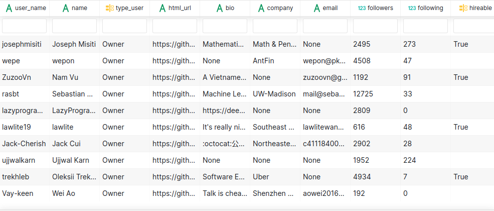
DataFrame? . . , .
, , :
, ?
, Matplotlib, , ( , ).
, Altair, Bokeh Plotly, , , .
? , Matplotlib, , , API. , Altair, , .
, , , , ?
, Github :
I Scraped more than 1k Top Machine Learning Github Profiles and this is what I Found
Datapane, Python API Python-. Datapane.
csv , Datapane Blob.
import datapane as dp
dp.Blob.get(name='github_data', owner='khuyentran1401').download_df()
Datapane, Blob. .
Matplotlib
Matplotlib, , Python . , data science, Matplotlib.
.
, 100 , Matplotlib :
import matplotlib.pyplot as plt
top_followers = new_profile.sort_values(by='followers', axis=0, ascending=False)[:100]
fig = plt.figure()
plt.bar(top_followers.user_name,
top_followers.followers)
- :
fig = plt.figure()
plt.text(0.6, 0.7, "learning", size=40, rotation=20.,
ha="center", va="center",
bbox=dict(boxstyle="round",
ec=(1., 0.5, 0.5),
fc=(1., 0.8, 0.8),
)
)
plt.text(0.55, 0.6, "machine", size=40, rotation=-25.,
ha="right", va="top",
bbox=dict(boxstyle="square",
ec=(1., 0.5, 0.5),
fc=(1., 0.8, 0.8),
)
)
plt.show()
Matplotlib , , .
, , , X Y, , Matplotlib .
correlation = new_profile.corr()
fig, ax = plt.subplots()
im = plt.imshow(correlation)
ax.set_xticklabels(correlation.columns)
ax.set_yticklabels(correlation.columns)
plt.setp(ax.get_xticklabels(), rotation=45, ha="right",
rotation_mode="anchor")
: Matplotlib , , .
Seaborn
Seaborn - Python , Matplotlib. , .
. , seaborn , matplotlib, .
, , .
correlation = new_profile.corr()
sns.heatmap(correlation, annot=True)
x y!
2.
seaborn , , , . ., , , . , , Matplotlib.
sns.set(style="darkgrid")
titanic = sns.load_dataset("titanic")
ax = sns.countplot(x="class", data=titanic)
Seaborn , matplotlib.
: Seaborn — Matplotlib . , , Matplotlib, seaborn (, , , . .), .
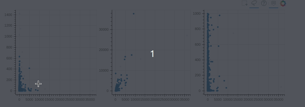
Plotly
Python Plotly . , Matplotlib seaborn, , , , . .
R
R Python, Plotly Python!
- Plotly Express, Python.
import plotly.express as px
fig = px.scatter(new_profile[:100],
x='followers',
y='total_stars',
color='forks',
size='contribution')
fig.show()
2.
Plotly . , .
, matplotlib? , Plotly
import plotly.express as px
top_followers = new_profile.sort_values(by='followers', axis=0, ascending=False)[:100]
fig = px.bar(top_followers,
x='user_name',
y='followers',
)
fig.show()
, , , . , .
3.
Plotly .
import plotly.express as px
import datapane as dp
location_df = dp.Blob.get(name='location_df', owner='khuyentran1401').download_df()
m = px.scatter_geo(location_df, lat='latitude', lon='longitude',
color='total_stars', size='forks',
hover_data=['user_name','followers'],
title='Locations of Top Users')
m.show()
, , . , - .
: Plotly .
Altair
Altair - Python , vega-lite, , .
1.
, , . , . , , , .
, . , , count() y_axis
import seaborn as sns
import altair as alt
titanic = sns.load_dataset("titanic")
alt.Chart(titanic).mark_bar().encode(
alt.X('class'),
y='count()'
)
2.
Altair .
, , , Plotly, Altair , .
hireable = alt.Chart(titanic).mark_bar().encode(
x='sex:N',
y='mean_age:Q'
).transform_aggregate(
mean_age='mean(age)',
groupby=['sex'])
hireable
, transform_aggregate()
(mean(age)
) (groupby=['sex']
) mean_age
). Y .
, - ( ), :N
, mean_age
- ( , ), :Q
.
3.
Altair , , .
, , . - :
brush = alt.selection(type='interval')
points = alt.Chart(titanic).mark_point().encode(
x='age:Q',
y='fare:Q',
color=alt.condition(brush, 'class:N', alt.value('lightgray'))
).add_selection(
brush
)
bars = alt.Chart(titanic).mark_bar().encode(
y='class:N',
color='class:N',
x = 'count(class):Q'
).transform_filter(
brush
)
points & bars
, , . , , , , - Python!
, , , , , , seaborn Plotly. Altair 5000 .
: Altair . Altair , 5000 , Plotly Seaborn.
Bokeh
Bokeh - , .
Matplotlib
, Bokeh, , Matplotlib.
Matplotlib , . Bokeh , ; , , Matplotlib, .
, Matplotlib,
import matplotlib.pyplot as plt
fig, ax = plt.subplots()
x = [1, 2, 3, 4, 5]
y = [2, 5, 8, 2, 7]
for x,y in zip(x,y):
ax.add_patch(plt.Circle((x, y), 0.5, edgecolor = "#f03b20",facecolor='#9ebcda', alpha=0.8))
#Use adjustable='box-forced' to make the plot area square-shaped as well.
ax.set_aspect('equal', adjustable='datalim')
ax.set_xbound(3, 4)
ax.plot() #Causes an autoscale update.
plt.show()
, Bokeh, :
from bokeh.io import output_file, show
from bokeh.models import Circle
from bokeh.plotting import figure
reset_output()
output_notebook()
plot = figure(plot_width=400, plot_height=400, tools="tap", title="Select a circle")
renderer = plot.circle([1, 2, 3, 4, 5], [2, 5, 8, 2, 7], size=50)
selected_circle = Circle(fill_alpha=1, fill_color="firebrick", line_color=None)
nonselected_circle = Circle(fill_alpha=0.2, fill_color="blue", line_color="firebrick")
renderer.selection_glyph = selected_circle
renderer.nonselection_glyph = nonselected_circle
show(plot)
2.
Bokeh . , , .
, 3 ,
from bokeh.layouts import gridplot, row
from bokeh.models import ColumnDataSource
reset_output()
output_notebook()
source = ColumnDataSource(new_profile)
TOOLS = "box_select,lasso_select,help"
TOOLTIPS = [('user', '@user_name'),
('followers', '@followers'),
('following', '@following'),
('forks', '@forks'),
('contribution', '@contribution')]
s1 = figure(tooltips=TOOLTIPS, plot_width=300, plot_height=300, title=None, tools=TOOLS)
s1.circle(x='followers', y='following', source=source)
s2 = figure(tooltips=TOOLTIPS, plot_width=300, plot_height=300, title=None, tools=TOOLS)
s2.circle(x='followers', y='forks', source=source)
s3 = figure(tooltips=TOOLTIPS, plot_width=300, plot_height=300, title=None, tools=TOOLS)
s3.circle(x='followers', y='contribution', source=source)
p = gridplot([[s1,s2,s3]])
show(p)
Bokeh - , , , Matplotlib, , Seaborn, Altair Plotly.
, , , , .
, :
from bokeh.transform import factor_cmap
from bokeh.palettes import Spectral6
p = figure(x_range=list(titanic_groupby['class']))
p.vbar(x='class', top='survived', source = titanic_groupby,
fill_color=factor_cmap('class', palette=Spectral6, factors=list(titanic_groupby['class'])
))
show(p)
, , :
from bokeh.transform import factor_cmap
from bokeh.palettes import Spectral6
p = figure(x_range=list(titanic_groupby['class']))
p.vbar(x='class', top='survived', width=0.9, source = titanic_groupby,
fill_color=factor_cmap('class', palette=Spectral6, factors=list(titanic_groupby['class'])
))
show(p)
, , Bokeh
: Bokeh - , , , . , , , .
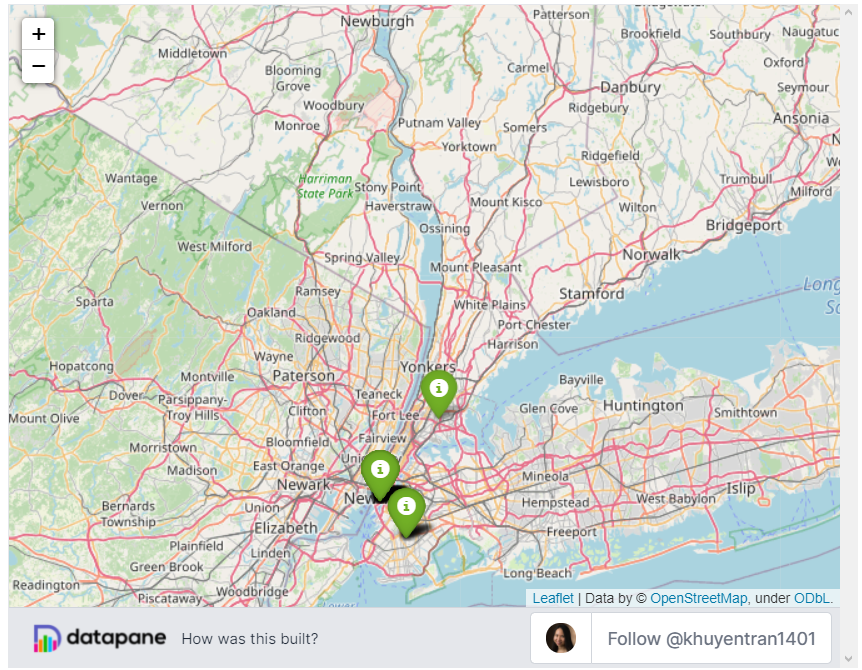
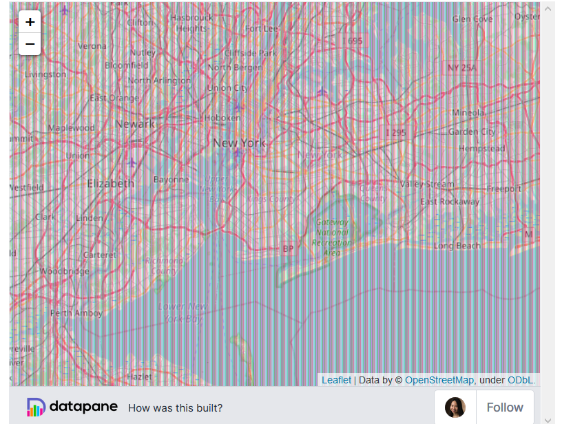
Folium
Folium . OpenStreetMap
, Mapbox Stamen
, Plotly, Altair Bokeh , Folium , - Google Map,
, Github Plotly? Folium:
import folium
# Load data
location_df = dp.Blob.get(name='location_df', owner='khuyentran1401').download_df()
# Save latitudes, longitudes, and locations' names in a list
lats = location_df['latitude']
lons = location_df['longitude']
names = location_df['location']
# Create a map with an initial location
m = folium.Map(location=[lats[0], lons[0]])
for lat, lon, name in zip(lats, lons, names):
# Create marker with other locations
folium.Marker(location=[lat, lon],
popup= name,
icon=folium.Icon(color='green')
).add_to(m)
m
2.
, Folium , :
# Code to generate map here
#....
# Enable adding more locations in the map
m = m.add_child(folium.ClickForMarker(popup='Potential Location'))
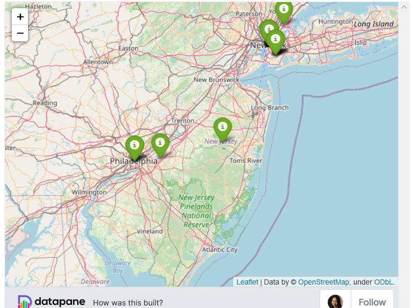
, , , .
3.
Folium , , Altair. , Github , , Github ? Folium :
from folium.plugins import HeatMap
m = folium.Map(location=[lats[0], lons[0]])
HeatMap(data=location_df[['latitude', 'longitude', 'total_stars']]).add_to(m)
, .
: Folium . Google Map.
! . , . .
, , , . , , , !
data science . LinkedIn Twitter.